TL;DR
In this blog, I explain the decisions and ideas that led me to train a Pose Control LoRA for Krea-2. The core architecture is a LoRA-based adaptation of Krea-2 with a modified input layer that accepts both the pose condition and the image latent. The final model release is the result of checkpoint interpolation between training steps 4000 and 4300.
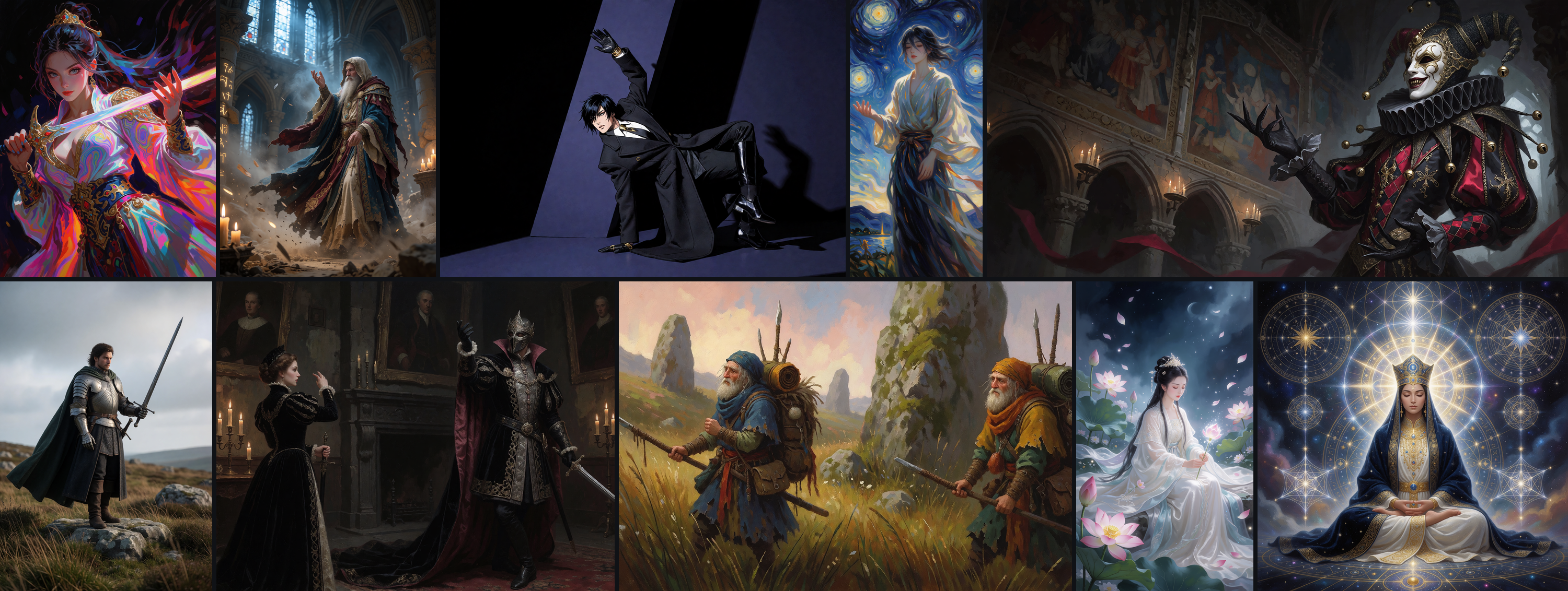
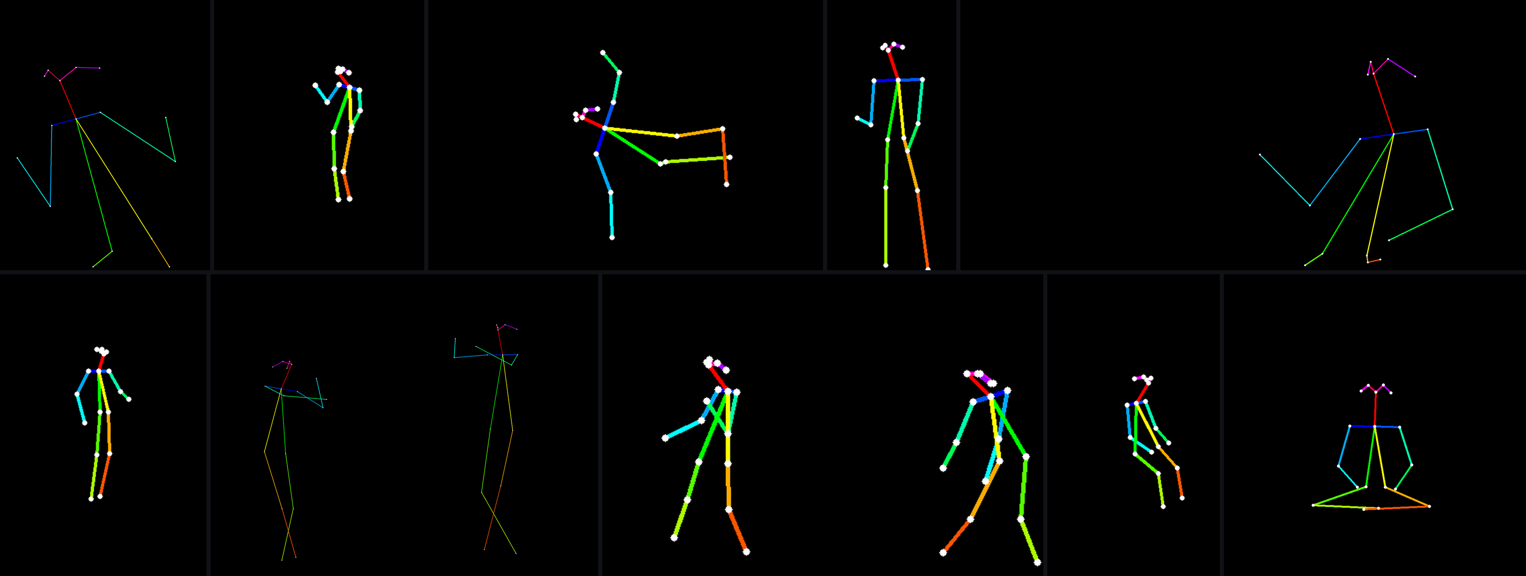
Figure 1 — Hero collage.
1. Introduction
Krea-2 is a 12B MMDiT-based open-weights image generation model focused on aesthetics and controllability through text and image inputs[1] . I recommend reading the Krea-2 Technical Report if you want a deeper understanding of the model and how it was trained.
Text-only generation does not give deterministic control over body layout, and pose is a useful conditioning signal because it helps separate geometry from appearance. The goal of this project is to use pose to control the broad body layout, while text controls identity, clothing, environment, and visual style.
This project builds on Tanmay Patil’s Krea-2 Depth ControlNet implementation[2] . I adapted that conditioning approach to human pose and built the dataset, preprocessing pipeline, training setup, evaluation pipeline, and inference path discussed below.
This is a fairly long blog, so in short, the following sections cover data preparation, architecture, the training objective, evaluations, results, and discussion.
2. Data Preparation
Data preparation ended up being one of the most time-consuming parts of the project. I spent around three weeks collecting, cleaning, captioning, and reviewing the data. Around 36k candidate images were collected initially, which were reduced to 17,495 image–pose–caption samples after pose generation and manual review.
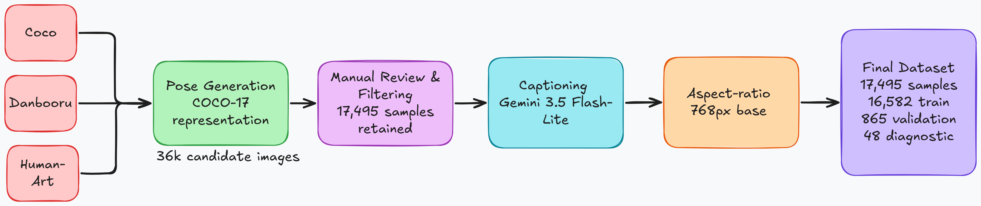
Figure 2 — Data Preparation Pipeline.
2.1 Dataset Collection
I collected data from COCO[5] , Danbooru[7] , and Human-Art[6] . The main goal was diversity in both pose and visual style.
COCO contributed photoreal images, Danbooru added anime images, and Human-Art provided paintings, sculptures, dance, and acrobatic poses. After pose generation, I manually reviewed the source image together with its corresponding pose condition and removed inaccurate or low-quality samples.
The final dataset contains 17,495 samples. Because of mixed licenses, I cannot share the complete dataset, but a portion is available on Hugging Face as PoseBridge, and the preprocessing pipeline is available on GitHub at PoseBridge Pre-processing.
Table 1 — Dataset Source Distribution
| Source | Images | Share |
|---|---|---|
| COCO | 3,893 | ~22.25% |
| Danbooru | 2,255 | ~12.89% |
| Human-Art Real Human | 3,257 | ~18.61% |
| Human-Art Painting | 6,502 | ~37.16% |
| Human-Art Sculpture | 1,588 | ~9.07% |
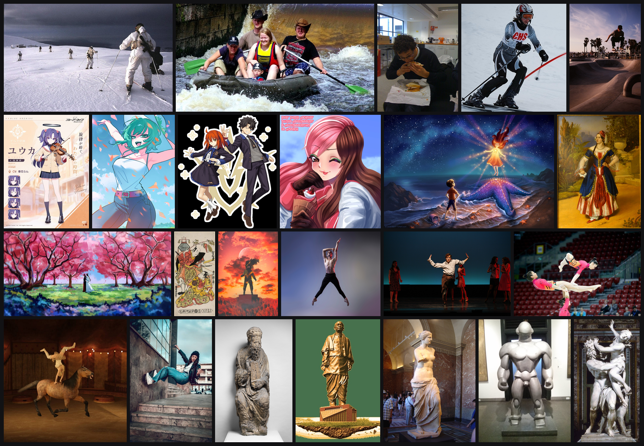
Figure 3 — Dataset montage.
2.2 Pose Representation
I experimented with richer pose representations, including hands and facial keypoints, but eventually standardized the dataset to the COCO 17-keypoint format.
Existing annotations from COCO and Human-Art were mapped to this representation. For Danbooru images, DWPose[8] was used to estimate the keypoints, followed by manual review of the generated pose conditions.
The final representation focuses on broad body structure rather than detailed hands, fingers, or facial expressions. The full keypoint and color mapping is available in Appendix A: Keypoints and Color Mapping.
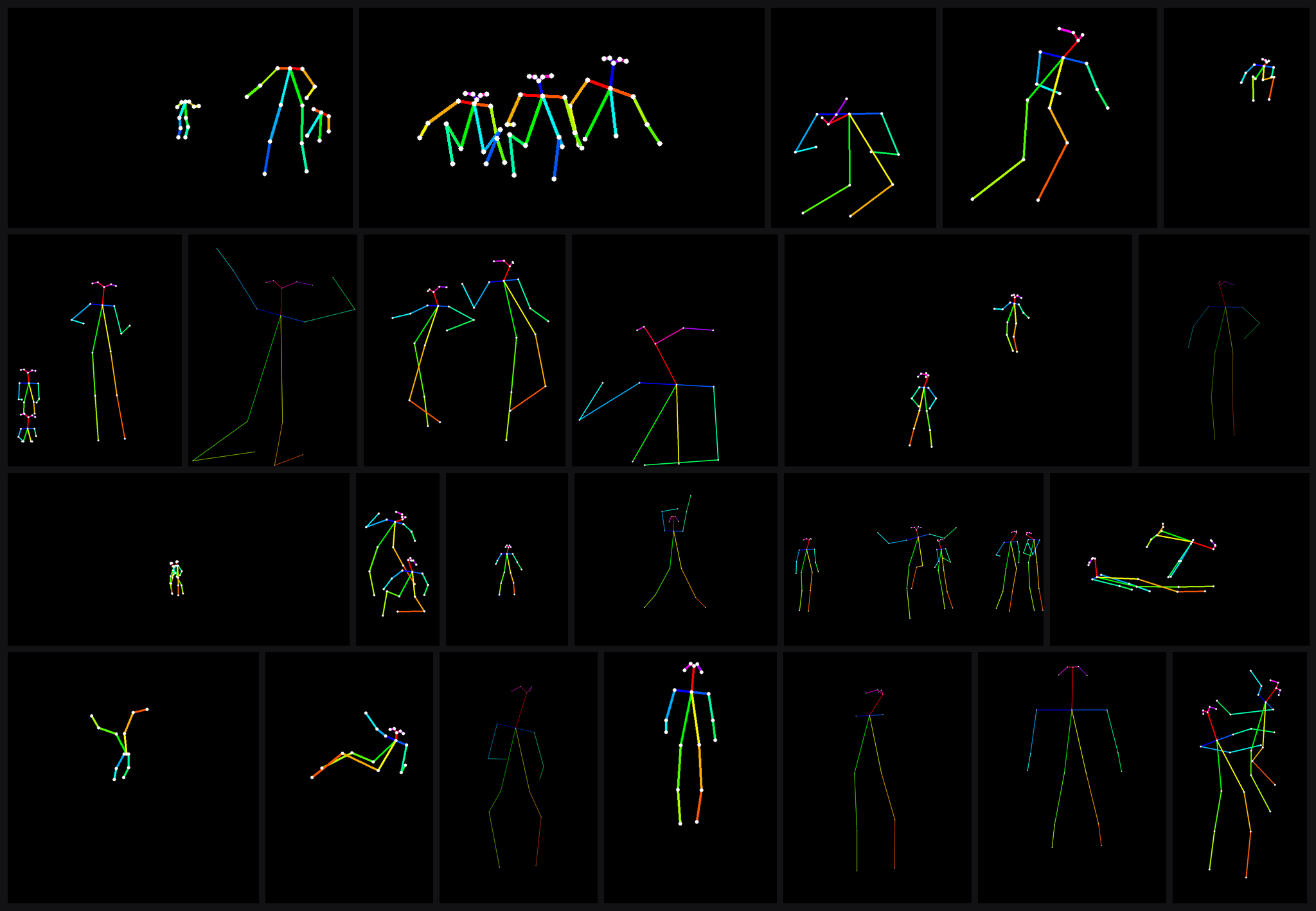
Figure 4 — Pose montage
2.3 Captioning
I initially tested BLIP[9]
and Qwen3-VL 3B[10]
for captioning, but the best results came from Gemini gemini-3.5-flash-lite[11]
. The total captioning cost was roughly $10.
The main goal was for captions to describe appearance, clothing, environment, and style without describing the subject’s pose or framing. The pose should come from the conditioning image rather than the text.
Pose-related and framing-related words were filtered from the generated captions. The complete filtering lists are included in the Appendix B: Caption Filtering Rules.
Example Caption
A photograph depicts a man with glasses wearing a dark green polo shirt and light-colored shorts next to a white and blue airplane on a concrete tarmac under a blue sky with white clouds, with green trees and a lamppost in the background, illuminated by bright daylight captured with a wide-angle lens, film grain
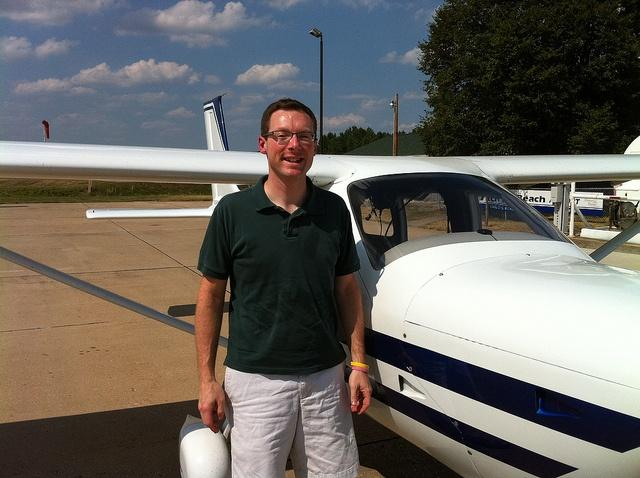
Figure 5 — Example image and generated caption.
2.4 Aspect-Ratio Buckets and Geometry
Instead of forcing every image into a square resolution, I used aspect-ratio buckets similar to the approach used in Tanmay Patil’s Krea-2 Depth ControlNet LoRA[2] .
Images were assigned to the nearest 768px-resolution bucket so that training could preserve more of the original image geometry. Table 2 — Dataset Aspect-Ratio Distribution
View table
| Category | Aspect Ratio Range | Images | Share |
|---|---|---|---|
| Square | $0.98 \le AR \le 1.02$ | 761 | 4.35% |
| Portrait | $0.50 < AR < 0.98$ | 8,854 | 50.61% |
| Landscape | $1.02 < AR < 2.00$ | 6,733 | 38.49% |
| Extreme Portrait | $AR \le 0.50$ | 1,001 | 5.72% |
| Extreme Landscape | $AR \ge 2.00$ | 146 | 0.83% |
| Total | All | 17,495 | 100.00% |
3. Architecture
The architecture was adapted from Tanmay’s Depth-Control Lora [2] which takes any image and a Depth map and adapts it to a new generation while preserving the same 3D structure. I followed the same pattern, but instead we give a pose skeleton, and it steers the image with a prompt towards the Pose. The Krea-2 Backbone is frozen; the only difference from the original Krea-2 is that the Input Layer is modified to take the Pose latent and image latent, rather than only the image latent.
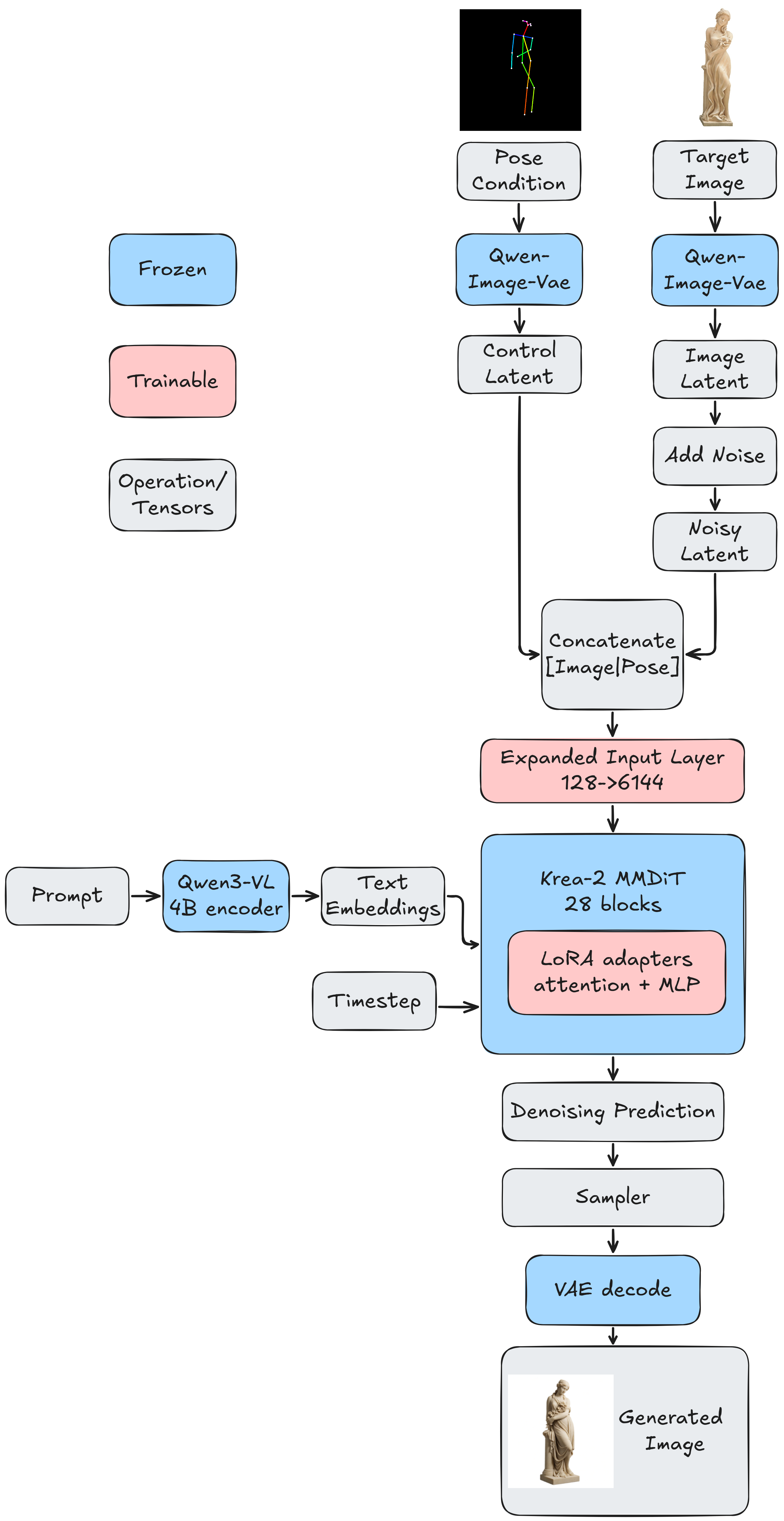
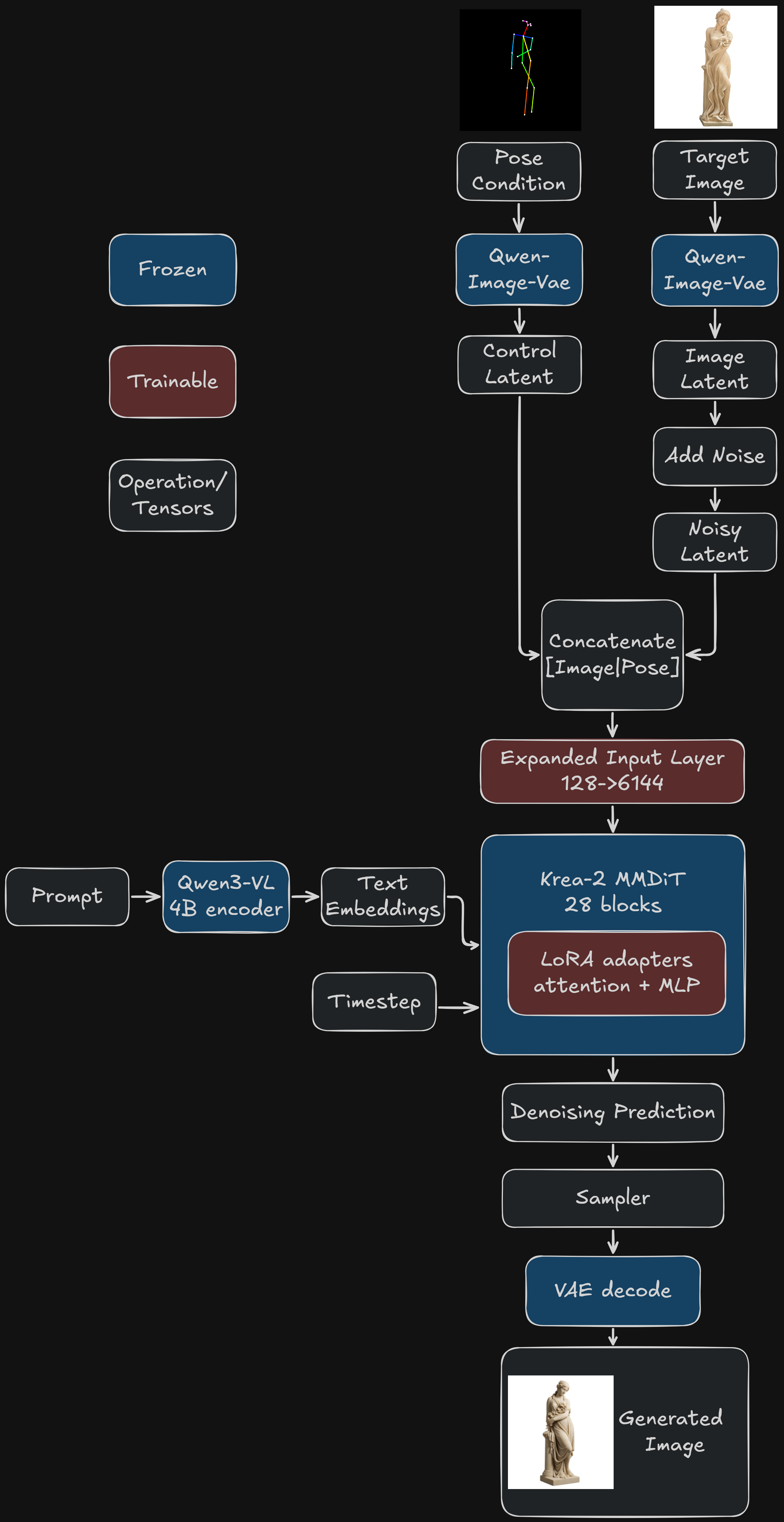
Figure 6 — Pose Control LoRA architecture for Krea-2.
3.1 Pose-Control Injection
The pose condition is encoded with the Qwen-Image VAE and kept as a clean control latent.
Training time
During training, the target image is encoded into a latent \(x_0\). Gaussian noise \(\epsilon\) is sampled and mixed with the image latent using the shifted timestep \(t\):
\[ x_t = t\epsilon + (1-t)x_0 \]The clean pose latent is then concatenated with \(x_t\). This doubles the input width from 64 to 128, so the original Krea-2 input projection is replaced with a trainable ControlInputLayer.
Inference time
At inference, there is no target image. Generation starts directly from Gaussian latent noise. At each denoising step, the current image latent is concatenated with the same clean pose latent before being passed through the expanded input layer.
The rest of Krea-2 remains frozen, while rank-64 LoRA[12] adapters are trained across all 28 transformer blocks. Only the expanded input layer and LoRA adapters are trainable.
3.2 Trainable Parameters
Direct fine-tuning of the full Krea-2 backbone is expensive, so I used parameter-efficient fine-tuning with LoRA. The final trainable state has 215.49 million parameters across 450 tensors. LoRA adapters use rank 64, targeting attn.{wq,wk,wv,gate,wo} and mlp.{gate,up,down} in all 28 transformer blocks. In addition to LoRA weights, the expanded control-input layer adds 792,576 parameters. Since Krea-2 has 13 billion parameters, this is about 1.66% of the full model.
Table 3 — Parameter Summary
| Component | Status | Parameters |
|---|---|---|
| Krea-2 backbone | Frozen | 0 trainable |
| Control input additions | Trainable | 792,576 |
| LoRA adapters | Trainable | 214,695,936 |
| Total trainable | — | 215,488,512 |
4. Training Objective and Training Strategy
4.1 Base Flow-Matching Objective
The Base Training Follows the standard flow-matching[13]
training methodology; the target image latent is noised at time step t. The pose-control latent stays clean. The model predicts the target velocity. The training uses MSE loss between the target and predicted velocity.
Equations
$$ x_t = t\epsilon + (1-t)x_0 $$$$ v = \epsilon - x_0 $$$$ L_{\text{flow}} = \operatorname{MSE}(\hat v, v) $$where:
- $x_0$ is the clean image latent
- $\epsilon$ is the sampled Gaussian noise
- $t$ is the sampled timestep
- $v$ is the target velocity
- $\hat v$ is the predicted velocity
4.2 Pose-Consistency Objective
The primary flow-matching loss, $L_{\text{flow}}$, does not explicitly account for body geometry or joint alignment. To address this, I introduced an additional pose-consistency objective that encourages the generated body geometry to follow the conditioning pose. This approach was inspired by ControlNet++[14] and was incorporated into the original training recipe.
The model first predicts the flow velocity $\hat{v}$ at timestep $t$. Using the noisy latent $x_t$ and the predicted velocity, it reconstructs an estimate of the clean image latent $\hat{x}_0$. For samples where pose supervision is active, the reconstructed image is decoded and passed through a frozen Keypoint R-CNN model[15] trained on COCO to estimate body keypoints.
The predicted joints and target joints are represented by:
$$\hat{p}_{\mathrm{norm}}, \qquad p_{\mathrm{norm}}$$Both are normalized to the person’s reference coordinate system before computing the Huber loss [18] . I use the Huber loss instead of mean squared error because it behaves quadratically for small errors while being less sensitive to large outliers.
The final training objective combines the original flow-matching loss with a small pose-consistency penalty. The pose-loss weight is set to $0.04$, encouraging better geometric adherence while retaining the original image-generation objective.
Note: Pose-consistency supervision was applied only to COCO and Human-Art samples after initial testing. Danbooru samples were trained using the standard flow-matching objective without the additional pose loss.
Equations
$$ \hat{x}_0 = x_t - t\hat{v} $$where
- $x_t$ = noisy image latent at timestep
- $\hat{v}$ = predicted velocity
- $t$= current timestep
- $\hat{x}_0$ = reconstructed estimate of the clean latent
- $\hat{p}_{\text{norm}}$ = normalized predicted joint coordinates
- $p_{\text{norm}}$ = normalized target joint coordinates
- $L_{\text{pose}}$ = penalty for pose mismatch
Table 4 — Pose-Consistency Training Settings
| Setting | Value |
|---|---|
| Pose-loss weight | λ_pose = 0.04 |
| Active timestep window | shifted t ∈ [0.10, 0.20] |
| Keypoints | 17 COCO body joints |
| Loss | Huber, delta = 1.0 |
| Pose estimator | frozen Keypoint R-CNN |
4.3 Training Recipe
The model was trained on Krea-2 Raw with the backbone frozen. The input projection (ControlInputLayer) was expanded to accept the concatenated image and pose-control latents, while rank-64 LoRA adapters were trained throughout the transformer. Training was performed on a single NVIDIA GH200 using BF16 autocast. A micro-batch size of 1 with 32 gradient-accumulation steps gave an effective batch size of 32.
Table 5 — Training Hyperparameters
| Setting | Frozen value |
|---|---|
| Base model | Krea-2 Raw |
| LoRA rank | 64 |
| Trainable parameters | 215,488,512 |
| Trainable tensor count | 450 |
| ControlInputLayer parameters | 792,576 |
| LoRA parameters | 214,695,936 |
| Optimizer | AdamW [19] |
| Betas | (0.9, 0.99) |
| Epsilon | 1e-8 |
| Weight decay | 0.0 |
| Max grad norm | 1.0 |
| Microbatch | 1 |
| Gradient accumulation | 32 |
| Effective batch | 32 |
| Caption dropout | 0.10 |
| Control dropout | 0.0 |
| Precision | CUDA BF16 autocast |
| Workers / prefetch | 4 / 4, persistent workers + pinned memory |
| Gradient checkpointing | Disabled |
torch.compile | Disabled |
| Fused AdamW | Disabled |
4.4 Training Stages
The total training time was 17 hours and 51 minutes. Training was done on Krea-2 Raw, while visual evaluations were performed using Krea-2 Turbo, following the setup recommended in the official Krea-2 repository [1]
.
The initial training ran for 3000 steps, with a 200-step warmup to 1e-4. From step 3000, the learning rate was cooled down until step 5000. I generated samples and compared the evaluation metrics every 100 steps, and step 4000 gave the best pose adherence.
For the final stage, I ran another cooldown from 2e-5 to 5e-6 until step 4500. After manually comparing the checkpoints at 100-step intervals, step 4300 looked better in terms of creativity, while step 4000 had better pose adherence.
The final release is an interpolation of these two checkpoints: 75% step 4000 + 25% step 4300, which gave the best overall result.
Table 6 — Training Stages and Learning-Rate Schedules
| Stage | Steps | LR schedule | Pose loss | Selected checkpoint |
|---|---|---|---|---|
| Initial production | 0→3000 | 200-step warmup to 1e-4, then 1e-4 | λ_pose = 0.04 | — |
| Cooldown | 3000→5000 | cosine 1e-4 → 1e-5 | λ_pose = 0.04 | parent-4000 |
| Finish-control | 4000→4500 | cosine 2e-5 → 5e-6 | λ_pose = 0.04 | A4300 |
| Final release | — | — | — | mix-025 |
4.5 Checkpoint Interpolation
The final release, as mentioned above, was the result of checkpoint interpolation. The interpolation was performed in FP32 over the trainable tensors from two selected checkpoints. The optimizer state, scheduler state, and training counters were not blended. Three interpolation ratios were evaluated: 25%, 50%, and 75%.
Equations
$$ \theta_{\alpha}=(1-\alpha)\theta_{\text{parent}}+\alpha\theta_{\text{A4300}} $$Candidates:
mix-025: ($\alpha$ = 0.25)mix-050: ($\alpha$ = 0.50)mix-075: ($\alpha$ = 0.75)
Final release:
$$ \text{mix-025} = 0.75\theta_{\text{parent-4000}} + 0.25\theta_{\text{A4300}} $$5. Experiments and Evaluation
5.1 Evaluation Protocol
I manually picked 48 images and conditions from trainset for Evals. As the Krea-2 report states I performed all evaluation on Krea-2 Turbo rather than Krea-2 Raw. I used the recommended settings from the Krea-2 Turbo repository for a all evaluations.
Table 7 — Evaluation Setup
| Item | Value |
|---|---|
| Evaluated images | 48 / 48 |
| Single-person images | 27 |
| Multi-person images | 21 |
| Renderer-qualified reference people | 101 |
| Eligible joints | 1,544 |
| Runtime | Krea-2 Turbo |
| Steps | 8 |
| CFG | 0 |
mu | 1.15 |
| Control scale | 1.0 |
5.2 Percentage of Correct Keypoints (PCK)
Percentage of Correct Keypoints (PCK) measures the fraction of predicted keypoints that fall within a normalized distance threshold of the corresponding ground-truth keypoints [16]
. The normalization makes the metric less sensitive to differences in person scale across images. A higher PCK score indicates better pose adherence, while a lower threshold makes the evaluation stricter. The evaluations were performed at three different thresholds: 0.05, 0.10, and 0.20.
PCK is globally pooled over all evaluated joints, and missing or unmatched reference joints are counted as failures. In my specific implementation, extra generated people are reported separately but do not directly reduce the PCK score.
I specifically chose PCK as an evaluation metric to measure the quality of pose adherence. However, I also manually inspected generations at each stage of training before proceeding to the next stage.
Equation
$$ \operatorname{PCK}@\tau = \frac{ \sum_{j \in E} \mathbf{1} [ \lVert r_j-g_j\rVert_2 \le \tau s_{p(j)} ] }{ |E| } $$where:
- ${E}$: the set of keypoints included in the evaluation.
- ${j}$: index of a keypoint in ${E}$.
- ${r_j}$: predicted/generated location of keypoint ${j}$.
- ${g_j}$: ground-truth/control location of keypoint ${j}$.
- $\lVert r_j-g_j\rVert_2$: Euclidean distance between the predicted and ground-truth locations.
- $\tau$: the normalized PCK threshold.
- $p(j)$: the person associated with keypoint $j$.
- $s_{p(j)}$: is the per-person normalization scale, defined as the diagonal of the axis-aligned extent of that person’s valid reference joints.
- $\mathbf{1}[\cdot]$: indicator function; it equals 1 when the condition is true and 0 otherwise.
- $|E|$: total number of evaluated keypoints.
5.3 CLIP Similarity
CLIP[17]
similarity score is the measure of image-prompt semantic aligment. The model used for this purpose is openai/clip-vit-base-patch32. The score calculated using simple cosine similarity formula using generated image and prompt embeddings. Note: CLIP score is Independent of PCK and stronger pose adherence does not necessarily imply higher CLIP similarity.
Equation
$$\operatorname{CLIPSim}(I,T)=\frac{f_I(I)\cdot f_T(T)}{\left\|f_I(I)\right\|_2\left\|f_T(T)\right\|_2}$$Where :
- $I$: Generated image
- $T$: Conditioning text prompt
- $f_I(I)$: CLIP image embedding
- $f_T(T)$: CLIP text embedding
- $\cdot$: Dot product
- $\|\cdot\|_2$: L2 norm
6. Results and Generations
6.1 Final Candidate Comparison
The result table below shows the comparison of evaluated metrics, and PCK metric which is used to determine the best generations indicates that mix-025 model outperforms all other models while maintaining moderate CLIP score.
Table 8 — Final Evaluation Results
| Candidate | PCK@.05 | PCK@.10 | PCK@.20 | CLIP |
|---|---|---|---|---|
| Turbo baseline | 0.0356 | 0.1101 | 0.3387 | 0.3440 |
| parent-4000 | 0.4301 | 0.5725 | 0.7105 | 0.3365 |
| mix-025 | 0.4521 | 0.6043 | 0.7241 | 0.3369 |
| A4300 | 0.4404 | 0.5939 | 0.7170 | 0.3370 |
6.2 Generations Across Different Conditions
The below figures are generations across different prompts and conditions of images.
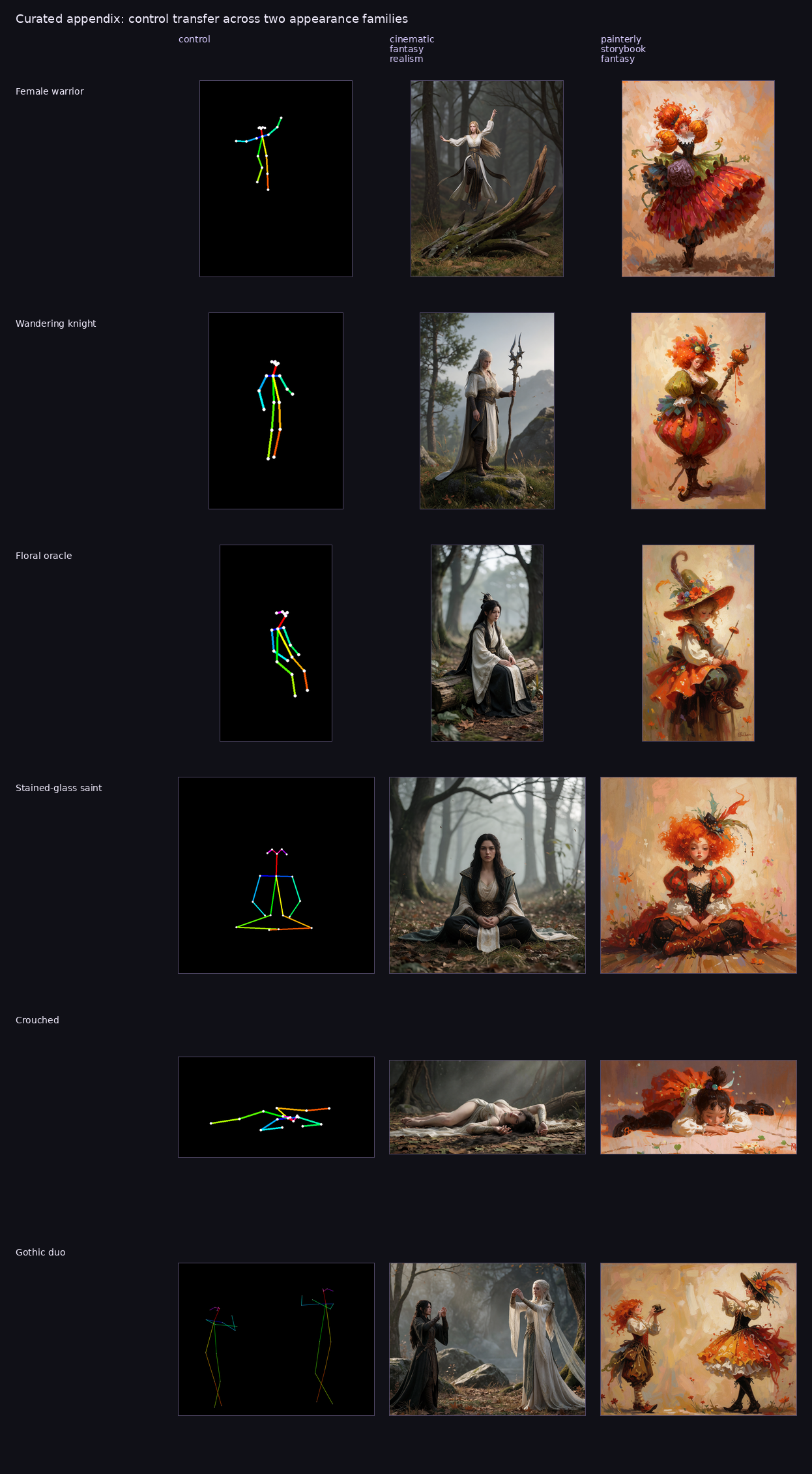
Figure 7 — Generations across different prompts and pose conditions.
6.3 Prompting Behavior
The pose conditioning controls the broad body geometry, while the text prompt determines the subject’s identity, appearance, clothing, environment, and visual style. The model is highly sensitive to prompting, particularly because it was trained on captions that intentionally excluded pose-related information. This separation encourages the model to follow the conditioning image for body geometry while relying on the text prompt for visual details.
For recommended prompting strategies and examples, refer to the Prompting Guide.
Note: The pose conditioning does not include hand or finger keypoints, so their positions and gestures are not directly controlled by the model.
7. Discussion and Limitations
7.1 What I Learned from This Project
I learned a great deal throughout this project, but if I had to identify the most challenging part, it would be data collection and preparation. This stage consumed most of my time. I manually reviewed every source image alongside its corresponding pose condition to ensure their accuracy and consistency (Even though the manual review was not absolutely necessary I did perform it because I wanted to have high quality data and I believe this careful data curation contributed significantly to the final model’s pose adherence.)
Another valuable lesson was the importance of overfitting a small batch. I followed Andrej Karpathy’s recommendation from A Recipe for Training Neural Networks[22] , using an overfitting test to examine whether my LoRA configuration had sufficient capacity to learn from a small set of examples. This helped me better understand the role of LoRA rank and the importance of validating the training setup before committing to a full training run.
I performed all data preprocessing on my local machine to minimize compute costs, while model training was carried out entirely on a single NVIDIA GH200. One of my biggest takeaways was the importance of designing evaluation metrics before writing the training script. Having a clear evals strategy setup from the beginning makes it much easier to understand whether the model is improving in the ways that actually matter.
Finally, I learned that checkpoint selection can be just as important as training longer. Experimenting with checkpoint interpolation was particularly interesting because it was an entirely new concept to me. It showed me how combining checkpoints from different stages of training could offer a better balance between pose adherence and creative flexibility.
7.2 Limitations
This project does have a couple of limitations and some of those are:
- There is no direct hand/finger control, and no face/expression control.
- The model still fails at certain multi-person cases which are harder to re-create.
- detector-based PCK does not measure complete visual quality
- The extra generated people are not directly penalized by PCK
- Prompt and control conflicts does reduce adherence to the pose
7.3 Experiments I Wanted to Try
There are a few experiments I wanted to try but did not fully commit to.
- I experimented with prompts in different languages, such as Chinese and Telugu, and observed an interesting behavior: depending on the language used, the model sometimes generated people wearing clothing associated with that culture, even without explicit style mentions [link to images and prompts]. I did not explore this behavior in depth, but one possible explanation could be biases or associations present in Qwen’s text embeddings.
- I also experimented with mixing the pose LoRA with existing LoRAs, such as style LoRAs. The model handled these combinations reasonably well and was still able to preserve pose control [link to images].
- I wanted to evaluate the effect of different LoRA ranks. The current model was trained and evaluated only with rank 64, so it would have been interesting to compare lower and higher ranks in terms of pose adherence, visual quality, and parameter efficiency.
- I also wanted to explore RL-based refinement for improving hands and facial expressions while still keeping them controllable through the prompt.
- I implemented ComfyUI workflow but I was not able to fully optimize it.
8. References and Acknowledgments
8.1 Acknowledgments
I would like to thank Naga Sai Abhinay for providing computational resources and offering valuable feedback throughout the project and on this blog.
I am grateful to Xuan Ju for providing me access to Human-Art dataset and to Tanmay Patil for open-sourcing his Krea-2 Depth ControlNet-LoRA implementation, which served as the architectural foundation for this project.
Finally, I thank all the dataset creators and researchers whose work helped me understand the underlying concepts and made this project possible.
8.2 AI Usage
Throughout the project, I used AI tools such as Codex to help write code and set up training scripts. I also used AI for grammar editing and checking the formatting of this blog. However, the technical content, experiments, decisions, and conclusions presented in the blog were not generated by AI.
8.3 References
- Lee, S., et al. (2026). Krea 2 Technical Report. Krea. Technical Report
- Patil, T. Krea-2 Depth ControlNet-LoRA. GitHub Repository
- Zhang, L., Rao, A., & Agrawala, M. (2023). Adding Conditional Control to Text-to-Image Diffusion Models. ICCV. Paper
- Cao, Z., Simon, T., Wei, S.-E., & Sheikh, Y. (2017). Realtime Multi-Person 2D Pose Estimation Using Part Affinity Fields. CVPR. Paper
- Lin, T.-Y., et al. (2014). Microsoft COCO: Common Objects in Context. ECCV. Paper
- Ju, X., Zeng, A., Wang, J., Xu, Q., & Zhang, L. (2023). Human-Art: A Versatile Human-Centric Dataset Bridging Natural and Artificial Scenes. CVPR. Paper
- Anonymous, Danbooru Community, & Branwen, G. (2022). Danbooru2021: A Large-Scale Crowdsourced & Tagged Anime Illustration Dataset. Dataset
- Yang, Z., Zeng, A., Yuan, C., & Li, Y. (2023). Effective Whole-Body Pose Estimation with Two-Stages Distillation. ICCV Workshops. Paper
- Li, J., Li, D., Xiong, C., & Hoi, S. (2022). BLIP: Bootstrapping Language-Image Pre-training for Unified Vision-Language Understanding and Generation. Paper
- Bai, S., et al. (2025). Qwen3-VL Technical Report. Paper
- Google DeepMind (2026). Gemini 3.5 Flash-Lite Model Card. Model Card
- Hu, E. J., et al. (2021). LoRA: Low-Rank Adaptation of Large Language Models. Paper
- Lipman, Y., Chen, R. T. Q., Ben-Hamu, H., Nickel, M., & Le, M. (2023). Flow Matching for Generative Modeling. ICLR. Paper
- Li, M., et al. (2024). ControlNet++: Improving Conditional Controls with Efficient Consistency Feedback. ECCV. Paper
- He, K., Gkioxari, G., Dollár, P., & Girshick, R. (2017). Mask R-CNN. ICCV. Paper
- Shrestha, R., Thakur, A. S., & Wang, C. (2026). Human Pose Estimation in 2D and 3D: A Survey of Analytical Methods, Benchmarking Frameworks, and Engineering Applications. Journal of Experimental and Theoretical Analyses, 4(3), 28. Paper
- Radford, A., et al. (2021). Learning Transferable Visual Models From Natural Language Supervision. ICML. Paper
- Huber, P. J. (1964). Robust Estimation of a Location Parameter. The Annals of Mathematical Statistics, 35(1), 73–101. Paper
- Loshchilov, I., & Hutter, F. (2019). Decoupled Weight Decay Regularization. ICLR. Paper
- Liu, X., Gong, C., & Liu, Q. (2022). Flow Straight and Fast: Learning to Generate and Transfer Data with Rectified Flow. Paper
- Lipman, Y., et al. (2024). Flow Matching Guide and Code. Paper
- Karpathy, A. (2019). A Recipe for Training Neural Networks. Andrej Karpathy Blog. Article
Appendix
A. Keypoints and Color Mapping
Table A1 — COCO Keypoints and Color Mapping
| Index | RGB Tuple | Color Name | Hue Family |
|---|---|---|---|
| 0 | (255, 0, 0) | Red | Red |
| 1 | (255, 85, 0) | Red-Orange | Orange |
| 2 | (255, 170, 0) | Orange-Yellow | Orange |
| 3 | (255, 255, 0) | Yellow | Yellow |
| 4 | (170, 255, 0) | Lime Green | Green |
| 5 | (85, 255, 0) | Bright Green | Green |
| 6 | (0, 255, 0) | Pure Green | Green |
| 7 | (0, 255, 85) | Spring / Mint Green | Cyan-Green |
| 8 | (0, 255, 170) | Turquoise | Cyan |
| 9 | (0, 255, 255) | Cyan / Aqua | Cyan |
| 10 | (0, 170, 255) | Sky Blue | Blue |
| 11 | (0, 85, 255) | Royal Blue | Blue |
| 12 | (0, 0, 255) | Pure Blue | Blue |
| 13 | (85, 0, 255) | Violet | Indigo / Violet |
| 14 | (170, 0, 255) | Purple-Magenta | Purple |
| 15 | (255, 0, 255) | Magenta / Fuchsia | Magenta |
| 16 | (255, 0, 170) | Hot Pink | Pink |
| 17 | (255, 0, 85) | Crimson / Pink-Red | Pink-Red |
B. Caption Filtering Rules
Pose Words
 POSE_WORDS = [
 "stand", "standing", "sit", "sitting", "seated", "seat", "kneel", "kneeling",
 "lying", "laying", "lay", "walk", "walking", "run", "running", "jump", "jumping",
 "crouch", "crouching", "bend", "bending", "bent", "lean", "leaning", "reach",
 "reaching", "stretch", "stretching", "pose", "posing", "gesture", "gesturing",
 "arms crossed", "legs crossed", "looking back", "over her shoulder",
 "over his shoulder", "turned", "twisted", "squat", "squatting", "hands on hips",
 "tiptoe", "dancing", "stance", "posture", "curled", "arched", "tilted", "propped",
 "straddling", "prone", "supine", "upright", "reclining", "hunched", "slouch",
 "raised arm", "raised arms", "outstretched", "mid-stride", "mid-flight",
 "extended forward", "riding", "ride", "astride", "mounted", "mounting", "perched",
]
Framing Words
FRAMING_WORDS = [
    "close-up", "close up", "medium shot", "wide shot", "full shot", "full-length shot",
    "medium close-up", "extreme close-up", "headshot", "head shot", "portrait shot",
    "portrait-style", "cowboy shot", "waist up", "waist-up", "knees up", "knees-up",
    "chest up", "shoulders up", "from the waist", "entire figure", "entire statue",
    "full body shot", "full-body shot", "full-length",
]
C. Additional Generations
The following figures illustrate how the same pose condition can produce different visual styles while preserving the underlying body geometry.
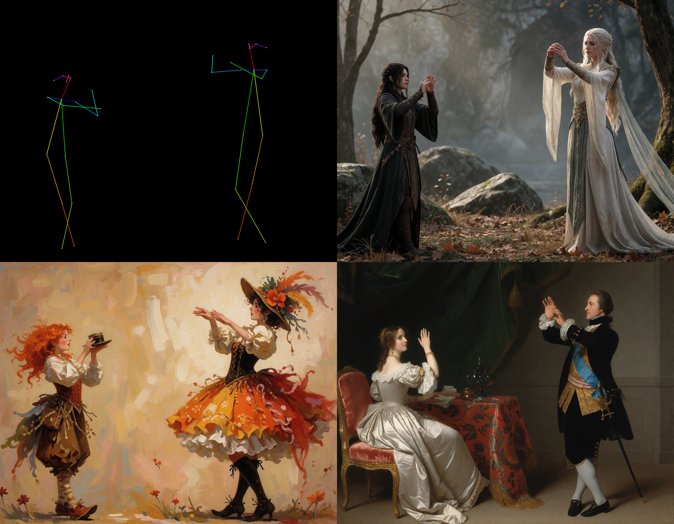
Figure C1 — Gothic duo: pose conditioning and generated images across different visual styles.
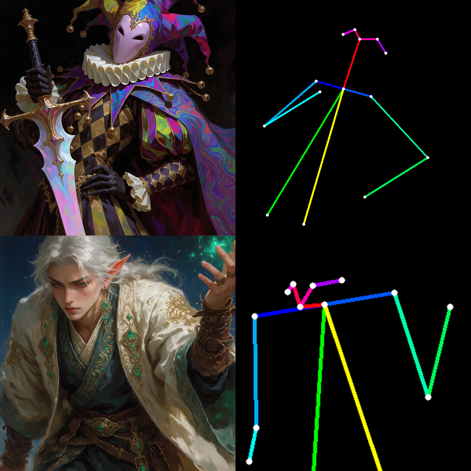
Figure C2 — Mage and jester: pose conditioning and corresponding generations.
The following collage presents additional generations across a variety of prompts, artistic styles, and visual compositions.
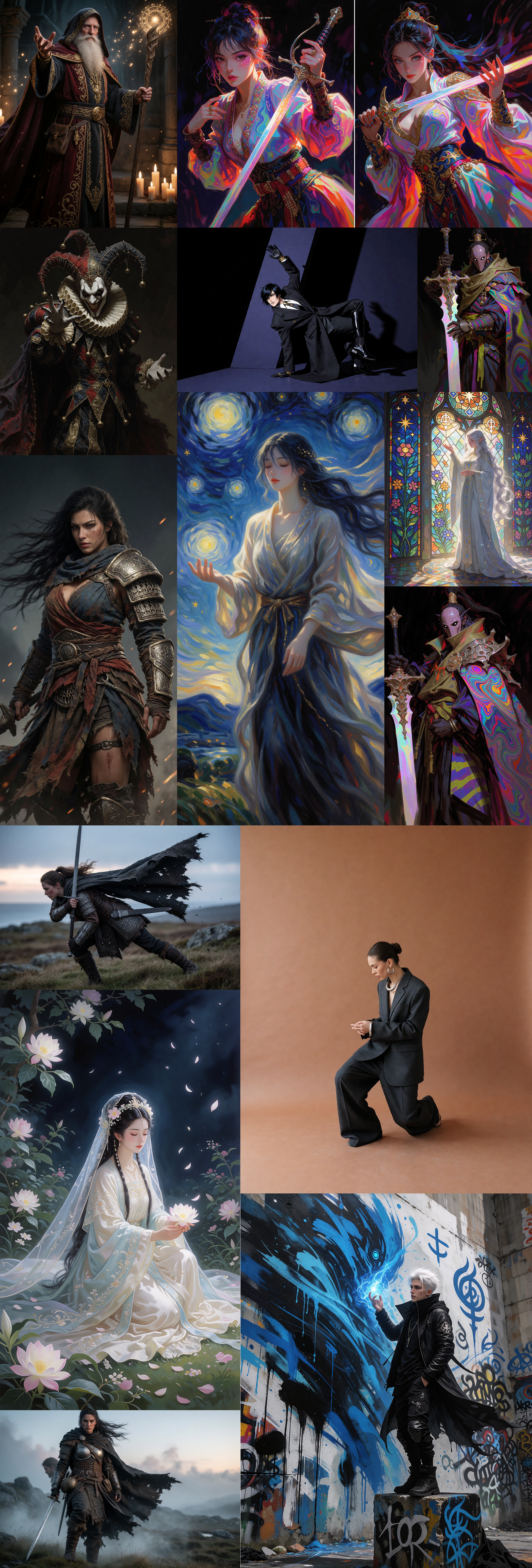
Figure C3 — Additional generations showcasing the model’s diversity across artistic styles and prompts.